
Introduction to Supply Elasticity
In economics, the concept of elasticity plays a fundamental role in understanding how markets respond to changing conditions. While elasticity of demand often receives significant attention, elasticity of supply is equally crucial in determining price dynamics, production adjustments, and market efficiency.
This primer explores the responsiveness of supply to price fluctuations – whether producers can quickly increase output when prices rise or if supply remains rigid despite market changes. By examining different degrees of elasticity, we can better analyze real-world markets, from commodities to financial assets.
Defining Elasticity of Supply
Elasticity of supply measures the percentage change in quantity supplied relative to a percentage change in price. It answers the question:
“If the price of a good increases by 1%, by what percentage does its supply increase?”
The formula for elasticity of supply (Es) is:

Where:
- Es = Elasticity of supply
- %ΔQs = Percentage change in quantity supplied
- %ΔP = Percentage change in price
Interpreting the Elasticity Coefficient
- If Es = ∞: Supply is perfectly elastic (infinite response at a fixed price)
- If Es > 1: Supply is elastic (responsive to price changes)
- If Es = 1: Supply is unit elastic (proportional response)
- If Es < 1: Supply is inelastic (limited response)
- If Es = 0: Supply is perfectly inelastic (no response)
Let’s go over various types of supply elasticity.
Perfectly Elastic Supply (Es = ∞)
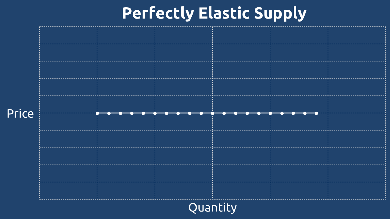
A perfectly elastic supply exists when producers are willing to supply any quantity of a good at a single, fixed price, but zero quantity if the price falls even slightly below that level. This represents an extreme case where the supply curve is completely horizontal, indicating infinite responsiveness to price changes at the equilibrium point.
Key Characteristics:
- Horizontal supply curve (zero slope)
- Infinite responsiveness: The slightest price drop eliminates all supply, while any quantity can be supplied at the equilibrium price.
- Theoretical in most markets, but approximated in highly competitive markets where firms are price takers (e.g., agricultural commodities traded at global prices).
Example Scenario:
If the market price for wheat is $5 per bushel, farmers may supply any amount demanded at that price. However, if the price dips to $4.99, they would supply zero wheat, as they cannot profit below the equilibrium price.
Elastic Supply (Eₛ > 1)
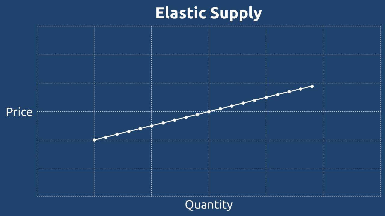
A good has an elastic supply when the percentage change in quantity supplied is greater than the percentage change in price. This means producers can quickly and significantly increase output when prices rise.
Key Characteristics:
- Relatively flat supply curve (low slope)
- High responsiveness: A small price increase leads to a large increase in quantity supplied.
- Common in industries with short production cycles (e.g., consumer goods), excess production capacity, easily available raw materials
Example Scenario:
If the price of smartphones increases by 10%, and manufacturers respond by increasing supply by 20%, the supply is elastic (Eₛ = 2).
Inelastic Supply (Eₛ < 1)
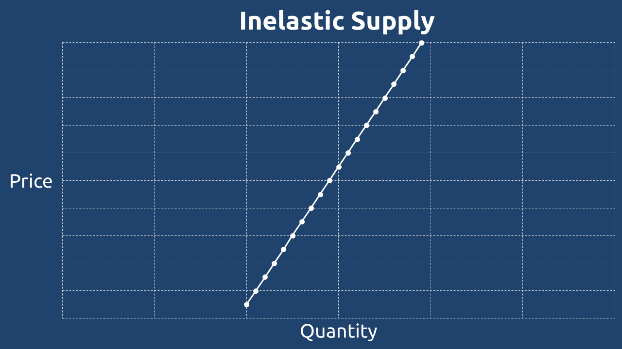
A good has an inelastic supply when the percentage change in quantity supplied is less than the percentage change in price. This indicates that producers cannot easily increase output, even when prices rise significantly.
Key Characteristics:
- Steep supply curve (high slope)
- Low responsiveness: Large price increases lead to only small increases in supply.
- Common in industries with long production lead times (e.g., oil, real estate), limited raw materials (e.g., rare minerals), high fixed costs (e.g., aircraft manufacturing)
Example Scenario:
If the price of crude oil increases by 20%, but producers can only increase supply by 5%, the supply is inelastic (Eₛ = 0.25).
Perfectly Inelastic Supply (Eₛ = 0)
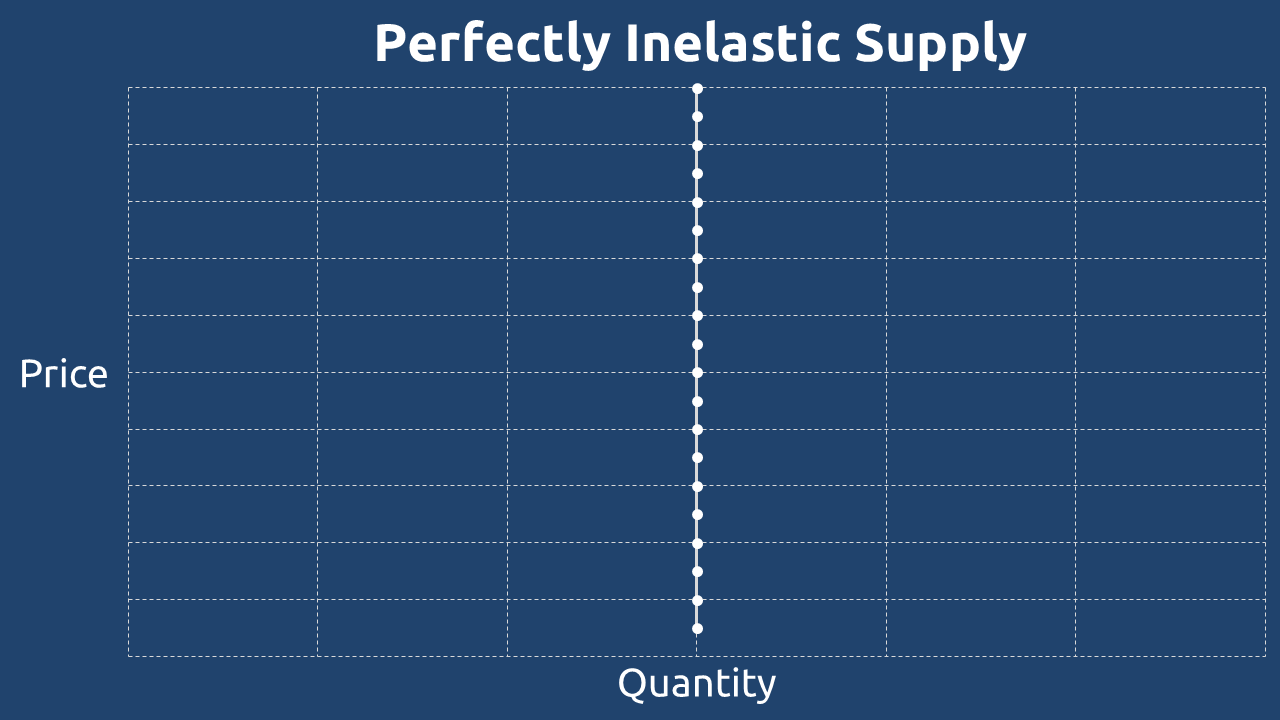
A perfectly inelastic supply exists when the quantity supplied does not change at all, regardless of price fluctuations. The supply curve is a vertical line, indicating zero responsiveness.
Key Characteristics:
- Vertical supply curve (infinite slope)
- Absolute rigidity: No change in supply even with extreme price changes.
- Rare in practice, but applies to fixed-quantity assets (e.g., land, original artworks)
Example Scenario:
If the price of a rare vintage painting increases by 500%, the supply remains one painting – it cannot be reproduced. Thus, supply is perfectly inelastic (Eₛ = 0).
After this brief primer on supply elasticity, we will now examine its practical implications across various money markets.