
This examination applies the concept of elasticity to modern monetary systems, contrasting the dynamic supply mechanisms of monies and money substitutes, including fiat currencies, government debt, precious metals, and cryptocurrencies. The analysis reveals that what many misinterpret as deflationary phenomena often stems from structural inelasticity rather than deliberate policy.
USD Elastic Supply
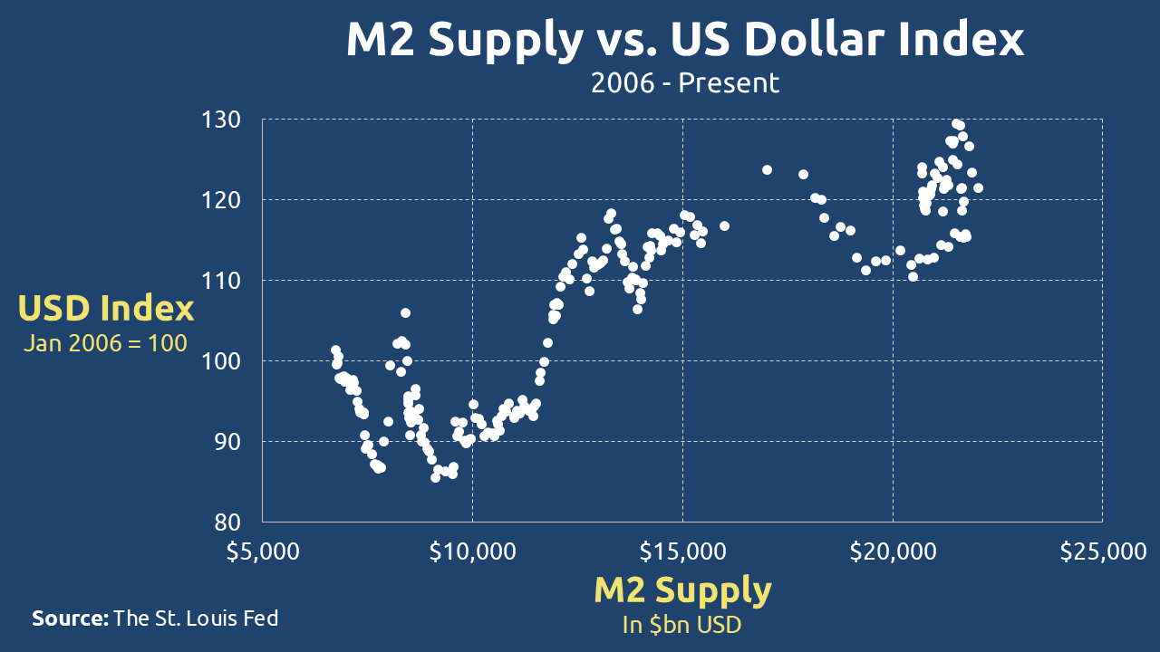
Like all contemporary fiat systems, the US dollar operates on a foundation of deliberate supply elasticity – a monetary superpower wielded through the Federal Reserve’s policy toolkit. Three primary mechanisms enable this flexibility:
- Open Market Operations – The Fed’s Treasury security purchases/sales directly modulate banking system liquidity
- Reserve Requirement Adjustments – Altering banks’ reserve ratios changes credit creation capacity
- Federal Funds Rate Targeting – Interest rate changes indirectly influence money multiplier effects
This institutional framework (visualized in Figure 1) grants the Fed extraordinary discretion – technically, the capacity for unlimited dollar creation, particularly evident during crisis interventions like 2008’s QE or pandemic-era stimulus.
Yet this elasticity faces natural boundaries:
- Inflationary Guardrails – Overexpansion risks currency debasement, as 1970s stagflation demonstrated
- Global Reserve Dynamics – Foreign central banks’ dollar holdings create external demand shocks
- Rate Transmission Limits – Higher borrowing costs eventually constrain money creation
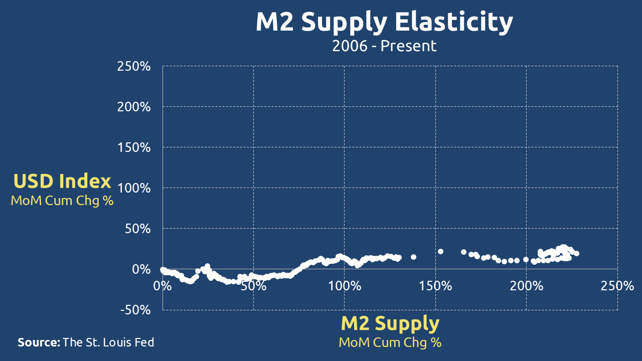
The M2 supply curve’s slope (Figure 2) perfectly encapsulates this tension – not perfectly horizontal like a theoretically infinite elastic supply, but sufficiently shallow to confirm the dollar’s engineered flexibility. Crucially, no statutory mechanism exists to prevent Fed balance sheet expansion when policymakers deem it necessary. This institutional reality positions the dollar as the ultimate elastic currency – a deliberately designed attribute that serves as both its greatest strength and most persistent vulnerability.
US Treasuries Elastic Supply
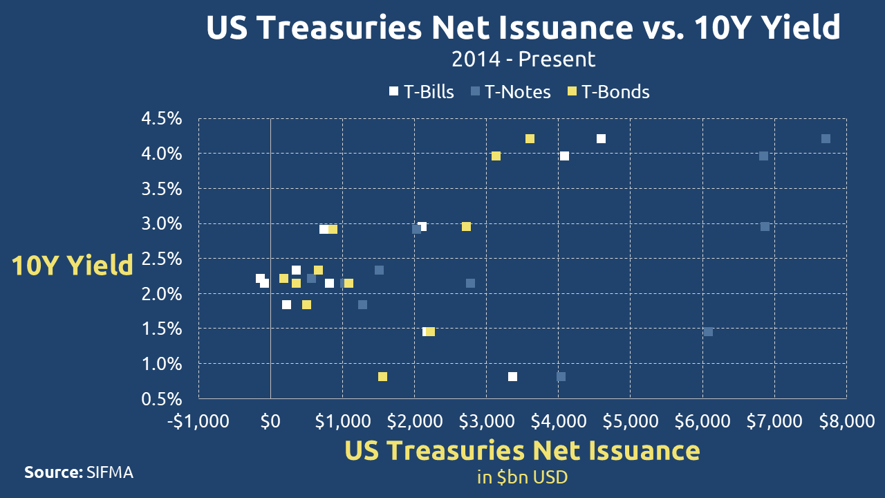
The supply dynamics of US Treasury instruments – including bills, notes, and bonds – exhibit fundamentally different characteristics across time horizons. In the immediate term, these securities demonstrate supply inelasticity, while their long-term behavior reveals inherent elasticity.
Short-Term Supply Rigidity
Three structural factors enforce temporary inelasticity:
- Predetermined Auction Calendar: The Treasury adheres to fixed issuance schedules, preventing real-time supply adjustments to demand volatility.
- Legislative Constraints: Debt ceiling limitations and congressional budget authorizations create hard boundaries on spontaneous debt issuance.
- Demand-Supply Decoupling: Even during periods of intense safe-haven demand (such as market crises), Treasury issuance volumes remain dictated by pre-established borrowing plans rather than market forces.
The Elasticity Inheritance
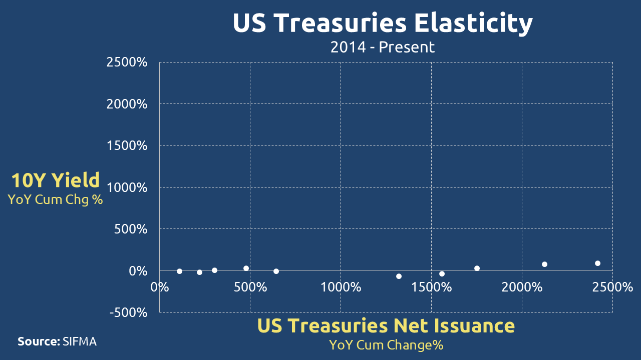
Treasuries ultimately derive their supply characteristics from their underlying foundation – the elastic US dollar. This relationship becomes particularly evident when examining longer timeframes. While short-term constraints exist, no immutable mechanisms permanently restrict debt expansion. This fundamental reality manifests clearly in Figure 3, where the near-horizontal trendline demonstrates the market’s absorption capacity for continuous debt issuance.
Fed’s Role (Quantitative Easing/Tightening):
- The Federal Reserve can artificially adjust supply elasticity by buying/selling Treasuries in open market operations.
- For example, during QE (Quantitative Easing), the Fed bought Treasuries, reducing market supply and lowering yields.
- Conversely, QT (Quantitative Tightening) increases market supply by letting bonds mature without reinvestment.
Beyond easily navigable procedural constraints, the Treasury market operates without substantive barriers to debt expansion. The nearly linear progression of net issuance from 2014-2024 provides empirical confirmation of this elastic supply paradigm. This trajectory underscores how Treasury securities, while appearing constrained in brief periods, ultimately function as flexible instruments of government financing over extended durations.
Gold’s Inelastic Supply
As a monetary substitute, gold presents a fascinating dichotomy in supply elasticity, with starkly contrasting interpretations between producers and economists.
The Producer Perspective: Theoretical Elasticity
Gold miners operate under the assumption of conditional elasticity – supply responds directly to price incentives. If market prices fall below extraction costs, producers rationally withhold supply by leaving gold deposits untouched, resulting in zero marginal production. This creates a price floor below which supply effectively disappears, mimicking characteristics of perfect elasticity within operational constraints.
The Economist Perspective: Structural Inelasticity
Macro analysts emphasize gold’s absolute supply constraints. Unlike fiat currencies, the Earth’s crust contains finite, physically limited gold reserves regardless of price fluctuations. This geological reality imposes fundamental inelasticity – no price surge can instantly create new deposits.
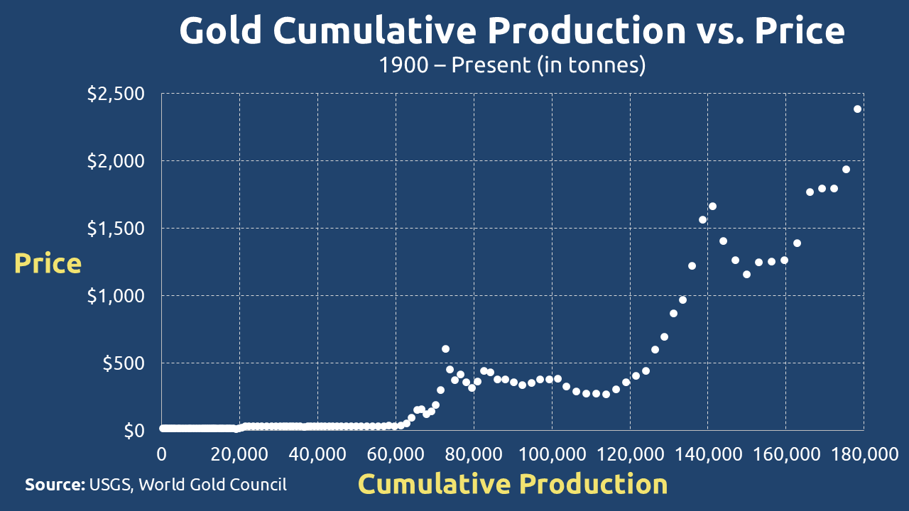
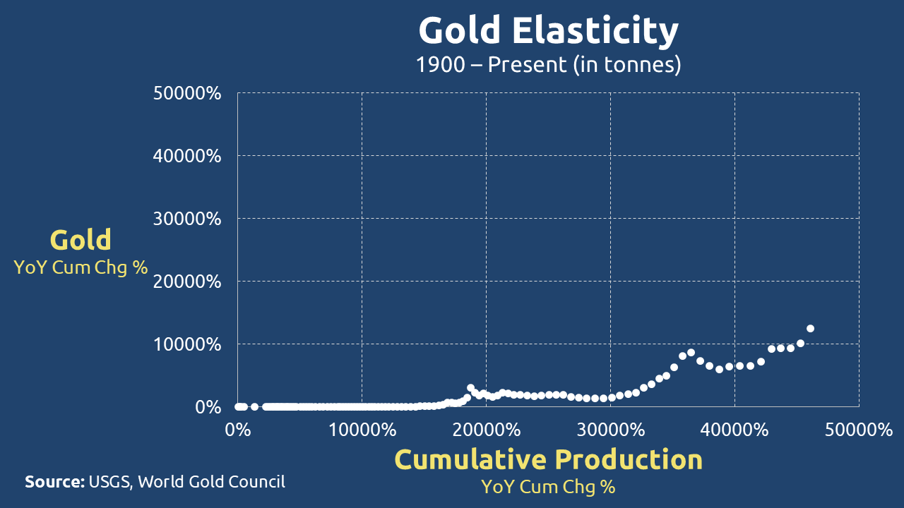
Gold’s supply dynamics reveal an interesting contradiction in practice. While the relationship between gold prices and annual production appears relatively stable at first glance (Figure 6), a closer examination shows the curve has actually been steepening since 2000, reflecting how inflationary pressures have impacted mining costs. This visual elasticity is somewhat misleading though – we need to separate short-term market behavior from gold’s fundamental nature.
In the immediate term, gold supply shows clear inelasticity because expanding production requires significant time and capital investment. The long-term picture seems more elastic at first, but this apparent flexibility is really just a reflection of humanity’s extraordinary gold rush over the past two centuries. Consider that all the gold ever mined would form a cube just 22 meters per side, with two-thirds of that total extracted since 1950 alone due to technological advances. While about 54,000-57,000 tonnes of economically viable reserves remain, this quantity is ultimately finite.
Two critical realities govern gold’s long-term supply:
- The total amount of accessible gold in the Earth’s crust is strictly limited.
- Even if more deposits exist, our ability to extract them faces technological and physical constraints.
These factors mean gold’s supply elasticity is ultimately constrained – it may appear flexible in certain timeframes, but its fundamental nature is decidedly inelastic when viewed through a long-term, geological lens. The temporary elasticity we observe is simply the mining industry catching up to centuries of accumulated demand, not evidence of truly elastic supply.
Bitcoin’s Inelastic Supply
Bitcoin presents perhaps the purest example of programmatically enforced supply inelasticity in monetary history. Its issuance schedule, hardcoded into the protocol since inception, remains completely unresponsive to market price fluctuations – a feature that stands in stark contrast to traditional commodities and fiat currencies. Some theorists even suggest this was intentional, pointing to the little-known but intriguing notion that Satoshi Nakamoto may have never intended Bitcoin to become a publicly traded asset in the first place.
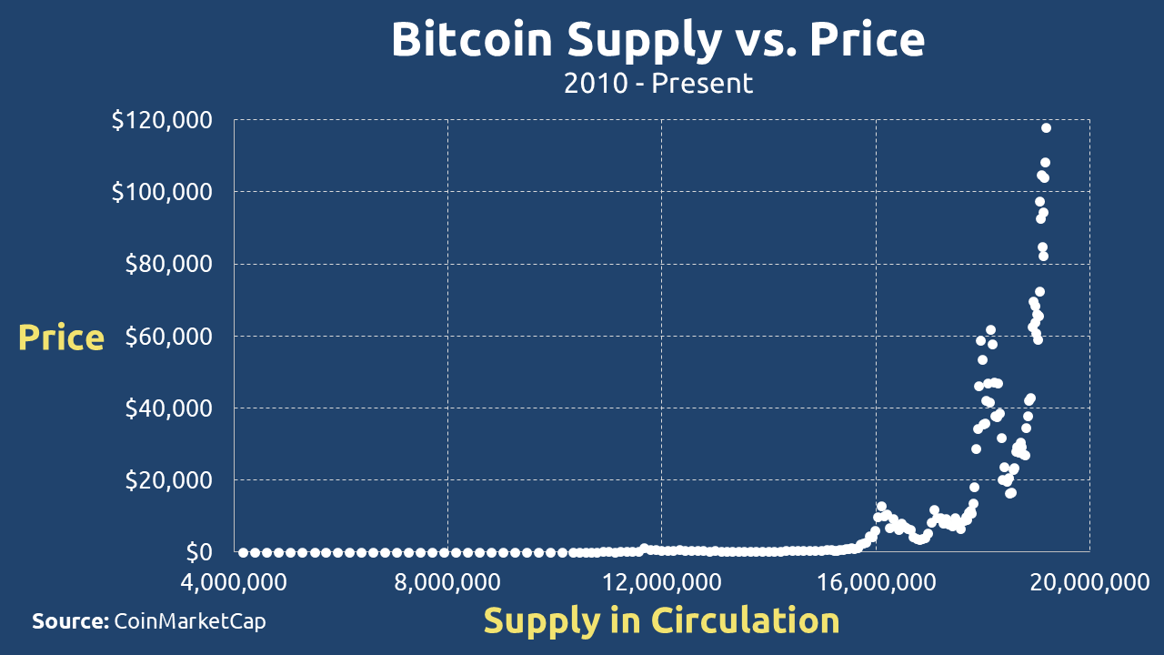
The supply dynamics become particularly interesting when examining Figure 7. At first glance, the pre-16 million BTC period might suggest some degree of supply elasticity, with the relatively flat curve appearing to show price responsiveness. However, this appearance is deceptive – the flattening simply reflects Bitcoin’s predetermined early-stage accelerated mining schedule, not any actual supply adjustment to market conditions.
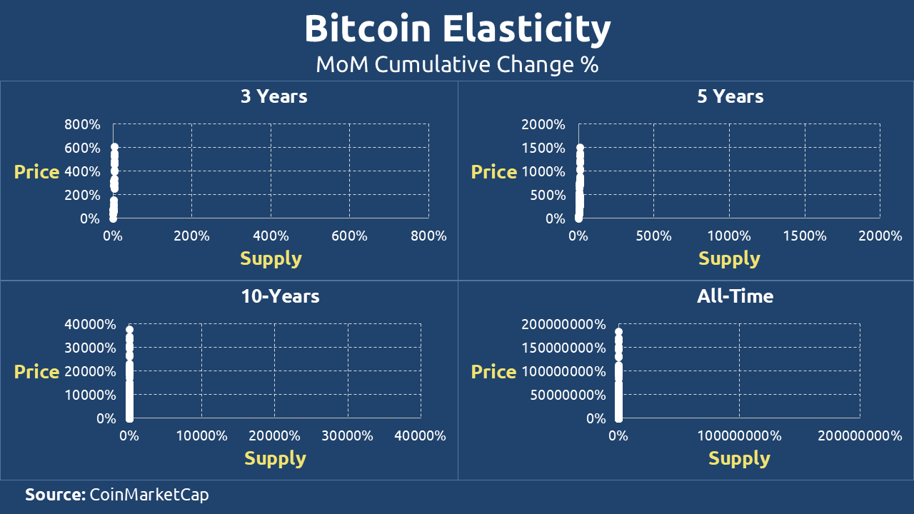
The true nature of Bitcoin’s inelasticity becomes undeniable when we examine the post-16 million coin era, particularly after Bitcoin’s first approach to the $20,000 price level. Despite subsequent price surges exceeding 300% in some periods, the mining algorithm continued its predetermined path without the slightest deviation. Figure 8 clearly demonstrates this through its characteristically steep slope – the unmistakable visual signature of a truly inelastic supply curve.
Looking ahead, Bitcoin’s supply characteristics will become even more extreme. Upon reaching its hardcoded limit of 21 million coins (expected around 2140), the system will transition to perfect inelasticity – a state where supply becomes completely fixed regardless of any price movements, market demands, or external economic conditions. This absolute supply cap represents what may be history’s first example of a monetary asset with mathematically guaranteed, permanently inelastic supply properties.
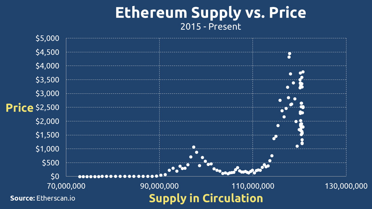
Ethereum’s Inelastic Supply
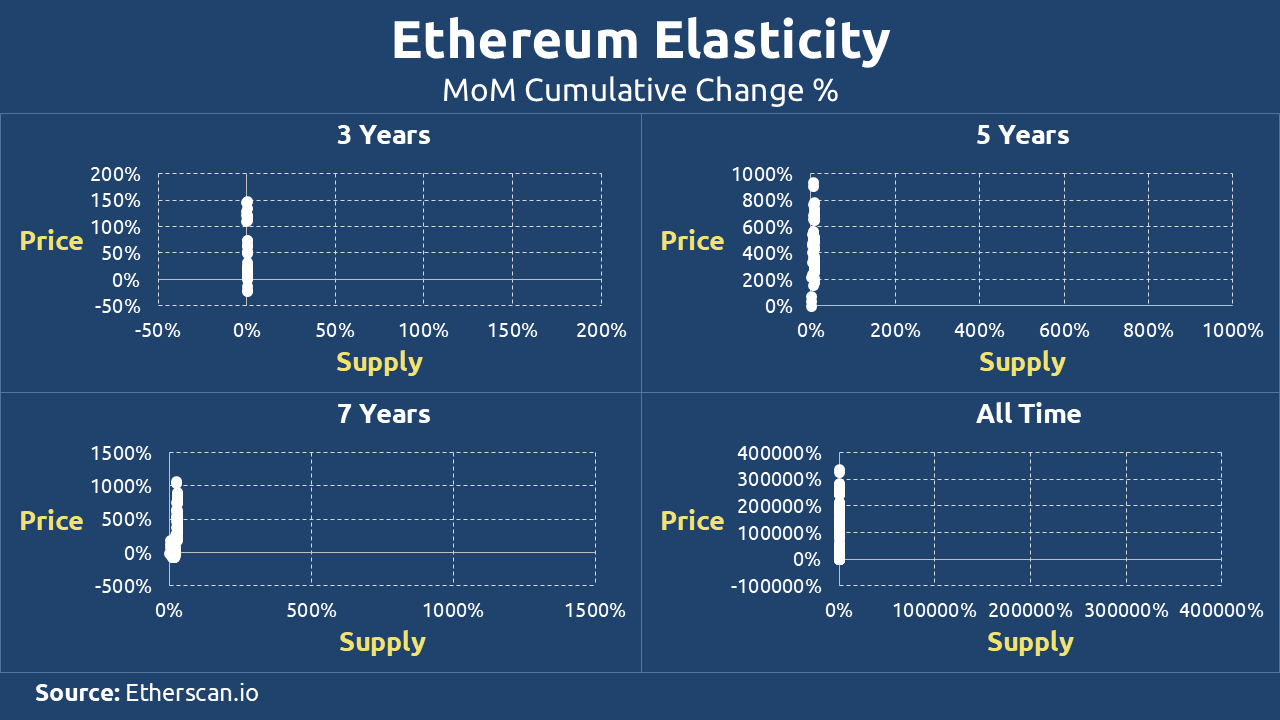
Like gold, Ethereum presents a fascinating monetary anomaly – a theoretically elastic asset behaving with apparent inelasticity. The numbers tell a striking story: from an initial 72 million ETH, supply has grown to just 121 million despite ETH’s price skyrocketing nearly 300,000%. This disconnect between price action and supply growth (evident in Figure 9) creates the visual illusion of vertical elasticity – a slope so steep it mimics Bitcoin’s hard-capped supply curve.
But this apparent inelasticity is an illusion. The London Fork’s introduction of ETH burning (Figure 10) created an artificial supply constraint, reducing annual inflation to a mere 0.7%. This mechanism operates through a precise equilibrium:

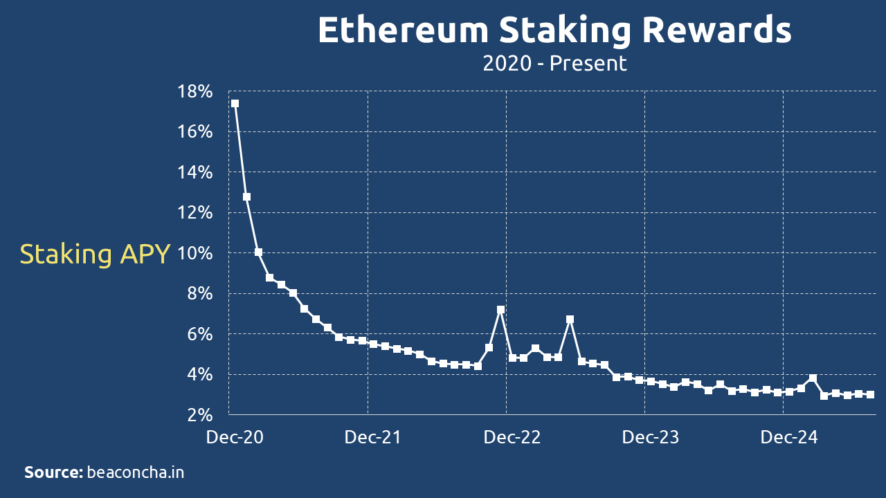
Herein lies Ethereum’s fragility. As staking yields have collapsed from 18% to under 3% in five years (Figure 11), the system faces compounding pressures:
- Validator Exodus Risk– Shrinking rewards may drive stake rotation to higher-yield chains
- Network Activity Dilemma– Reduced transactions mean lower fee revenue, further squeezing rewards
- Inflation Tradeoff– Preserving yields would require reducing burns, reawakening ETH’s inflationary nature
Ethereum’s current pseudo-inelasticity isn’t a fundamental property – it’s a temporary state sustained by network effects and careful fee market calibration. Like a dam holding back elastic potential energy, the system maintains stability only through constant protocol adjustments. When either adoption growth slows or validator patience wears thin, Ethereum’s underlying elasticity may reassert itself with potentially disruptive consequences.
This delicate balance makes Ethereum monetary policy’s most ambitious experiment – an elastic asset masquerading as hard money, sustained not by code-enforced scarcity but by continuous economic fine-tuning. Whether this equilibrium can endure remains crypto’s most consequential open question.
Visual evidence in Figures 9-10 shows the system’s current stability, but the steepening yield curve on Figure 11 suggests growing structural tensions.
Summary
When evaluating modern monetary instruments, it becomes critically important to examine supply elasticity through temporal lenses – short-term reactivity and long-term structural tendencies. This dual-axis analysis reveals fundamental truths about how different assets respond (or refuse to respond) to market forces and institutional pressures.
| Money Type | Short-term | Long-term |
| Fiat | Elastic | Elastic |
| Treasuries | Inelastic | Elastic |
| Gold | Inelastic | Inelastic |
| Bitcoin | Inelastic | Perfectly Inelastic |
| Ethereum | Elastic | Elastic |
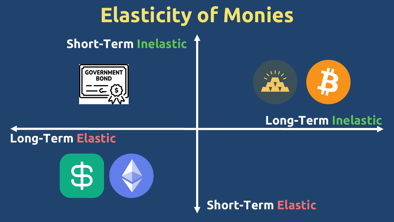
Figure 12 provides a systematic classification that crystallizes preceding discussions:
- Fiat Currencies (USD/EUR) maintain elastic properties across all time horizons, with central banks acting as perpetual supply adjusters.
- Treasury Securities display a unique temporal duality – their short-term inelasticity (constrained by auction schedules and debt ceilings) gives way to long-term elasticity.
- Gold’s double inelasticity – evident in both its geological constraints and production lead times—positions it as the natural antithesis to fiat systems.
- Bitcoin progresses from algorithmic inelasticity to perfect supply rigidity at its 21 million cap, creating the vertical supply curve.
- Ethereum’s current elastic-but-restrained state represents perhaps the most complex case – a system attempting to mimic Bitcoin’s scarcity while retaining flexibility.
This analytical structure inevitably prompts critical examination of GHOST’s position within the elasticity continuum – a fundamental consideration we will explore thoroughly in subsequent analysis.